
Open Excel Starter and take a look around
Open Excel Starter with the Windows Start button.
- Click the Start button . If Excel Starter is not included among the list of programs you see, click All Programs, and then click Microsoft Office Starter.
- Click Microsoft Excel Starter 2010.The Excel Starter startup screen appears, and a blank spreadsheet is displayed. In Excel Starter, a spreadsheet is called a worksheet, and worksheets are stored in a file called a workbook. Workbooks can have one or more worksheets in them.

1. Columns (labeled with letters) and rows (labeled with numbers) make up the cells of your worksheet.
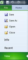
2. Clicking the File tab opens the Backstage view of your workbook, where you can open and save files, get information about the current workbook, and perform other tasks that do not have to do with the content of the workbook, such as printing it or sending a copy of it in e-mail.
3. Each tab in the ribbon displays commands that are grouped by task. You'll probably spend most of your time using the Home tab, when you're entering and formatting data. Use the Insert tab to add tables, charts, pictures, or other graphics to your worksheet. Use the Page Layout tab to adjust margins and layout, especially for printing. Use the Formulas tab to make calculations on the data in your worksheet.
4. The pane along the side of the Excel Starter window includes links to Help and shortcuts to templates and clip art, to give you a head-start on creating workbooks for specific tasks, such as managing a membership list or tracking expenses. The pane also displays advertising and a link to purchase a full-feature edition of Office.
Top of Page
Create a new workbook
When you create a workbook in Microsoft Excel Starter 2010, you can start from scratch or you can start from a template, where some of the work is already done for you.
- Click File, and then click New.
- If you want to start with the equivalent of a blank grid, click Blank workbook.
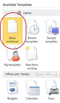 If you want a head-start on a particular kind of workbook, choose one of the templates available on Office.com. Choose from budgets, event planners, membership lists, and more.
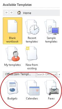
- Excel Starter opens the blank workbook or template, ready for you to add your data.
Top of Page
Save a workbook
When you interrupt your work or quit, you must save your worksheet, or you will lose your work. When you save your worksheet, Excel Starter creates a file called a workbook, which is stored on your computer.
- Click the Save button
 on the Quick Access Toolbar.(Keyboard shortcut: Press CTRL+S.)If this workbook was already saved as a file, any changes you made are immediately saved in the workbook, and you can continue working.
 - If this is a new workbook that you have not yet saved, type a name for it.
- Click Save.
Top of Page
Enter data
To work with data on a worksheet, you first have to enter that data in the cells on the worksheet.
- Click a cell, and then type data in that cell.
- Press ENTER or TAB to move to the next cell.Tip To enter data on a new line in a cell, enter a line break by pressing ALT+ENTER.
- To enter a series of data, such as days, months, or progressive numbers, type the starting value in a cell, and then in the next cell type a value to establish a pattern.For example, if you want the series 1, 2, 3, 4, 5..., type 1 and 2 in the first two cells.Select the cells that contain the starting values, and then drag the fill handle
 across the range that you want to fill.Tip To fill in increasing order, drag down or to the right. To fill in decreasing order, drag up or to the left.
Top of Page
Make it look right
You can format text and cells to make your worksheet look the way you want.
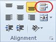
- To wrap text in a cell, select the cells that you want to format, and then on the Home tab, in the Alignment group, click Wrap Text.
- To adjust column width and row height to automatically fit the contents of a cell, select the columns or rows that you want to change, and then on the Home tab, in the Cells group, click Format.
 Under Cell Size, click AutoFit Column Width or AutoFit Row Height.Tip To quickly autofit all columns or rows in the worksheet, click the Select All button, and then double-click any boundary between two column or row headings.
- To change the font, select the cells that contain the data that you want to format, and then on the Home tab, in the Font group, click the format that you want.
- To apply number formatting, click the cell that contains the numbers that you want to format, and then on the Home tab, in the Number group, point to General, and then click the format that you want.
For more help with entering and formatting data, see Quick start: Format numbers in a worksheet.
Top of Page
Copy, move, or delete data
You can use the Cut, Copy, and Paste commands to move or copy rows, columns, and cells. To copy, press CTRL+C to use the Copy command. To move, press CTRL+X to use the Cut command.
- Select the rows, columns, or cells you want to copy, move, or delete.To select a row or column, click the row or column heading.
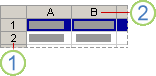 1. Row heading2. Column headingTo select a cell, click the cell. To select a range of cells, click click and drag, or click and use the arrow keys while holding down the SHIFT key.
 - Press CTRL+C to copy or CTRL+X to cut.If you want to delete a row or column, pressing DELETE while the row or columns is selected clears the contents, leaving an empty row or cell. To delete a row or column, right-click the row or column heading, and then click Delete Row or Delete Column.Note Excel displays an animated moving border around cells that have been cut or copied. To cancel a moving border, press ESC.
- Position the cursor where you want to copy or move the cells.To copy or move a row or column, click the row or column header that follows where you want to insert the row or column you copied or cut.To copy or move a cell, click the cell where you want to paste the cell you copied or cut.To copy or move a range of cells, click the upper-left cell of the paste area.
- Paste the data in the new location.For rows or columns, right-click the row or column heading at the new location, and then click the Insert command.For a cell or range of cells, press CTRL+V. The cells you copied or cut replace the cells at the new location.
For more information about copying and pasting cells, see Move or copy cells and cell contents
Top of Page
Change the order
When you sort information in a worksheet, you can see data the way you want and find values quickly.
Select the data that you want to sort
Use the mouse or keyboard commands to select a range of data, such as A1:L5 (multiple rows and columns) or C1:C80 (a single column). The range can include titles that you created to identify columns or rows.
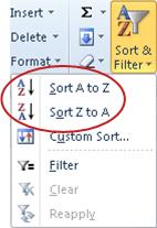
To sort with just two mouse clicks, click Sort & Filter, and then click either of the Sort buttons.
- Select a single cell in the column on which you want to sort.
- Click the top button to perform an ascending sort (A to Z or smallest number to largest).
- Click the bottom button to perform a descending sort (Z to A or largest number to smallest).
Top of Page
Filter out extra information
By filtering information in a worksheet, you can find values quickly. You can filter on one or more columns of data. You control not only what you want to see, but also what you want to exclude.
- Select the data that you want to filter
- On the Home tab, in the Edit group, click Sort & Filter, and then click Filter.
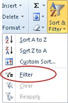
- Click the arrow
 in the column header to display a list in which you can make filter choices.Note Depending on the type of data in the column, Excel Starter displays either Number Filters or Text Filters in the list.
For more help with filtering, see Quick start: Filter data by using an AutoFilter.
Top of Page
Calculate data with formulas
Formulas are equations that can perform calculations, return information, manipulate the contents of other cells, test conditions, and more. A formula always starts with an equal sign (=).
Formula
|
Description
|
|---|---|
=5+2*3
|
Adds 5 to the product of 2 times 3.
|
=SQRT(A1)
|
Uses the SQRT function to return the square root of the value in A1.
|
=TODAY()
|
Returns the current date.
|
=IF(A1>0)
|
Tests the cell A1 to determine if it contains a value greater than 0.
|
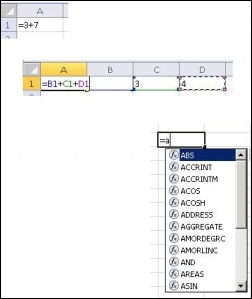
Select a cell and start typing
In a cell, type an equal sign (=) to start the formula.
Fill in the rest of the formula
- Type a combination of numbers and operators; for example, 3+7.
- Use the mouse to select other cells (inserting an operator between them). For example, select B1 and then type a plus sign (+), select C1 and type +, and then select D1.
- Type a letter to choose from a list of worksheet functions. For example, typing "a" displays all available functions that start with the letter "a."
Complete the formula
To complete a formula that uses a combination of numbers, cell references, and operators, press ENTER.
To complete a formula that uses a function, fill in the required information for the function and then press ENTER. For example, the ABS function requires one numeric value — this can be a number that you type, or a cell that you select that contains a number.
Top of Page
Chart your data
A chart is a visual representation of your data. By using elements such as columns (in a column chart) or lines (in a line chart), a chart displays series of numeric data in a graphical format.
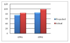
The graphical format of a chart makes it easier to understand large quantities of data and the relationship between different series of data. A chart can also show the big picture so that you can analyze your data and look for important trends.
- Select the data that you want to chart.
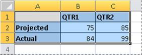 Tip The data should be arranged in rows or columns, with row labels to the left and column labels above the data — Excel automatically determines the best way to plot the data in the chart.
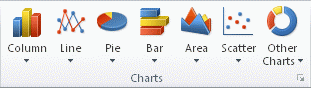
 - On the Insert tab, in the Charts group, click the chart type that you want to use, and then click a chart subtype.
 Tip To see all available chart types, click
 to launch the Insert Chart dialog box, and then click the arrows to scroll through the chart types.
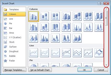
- When you rest the mouse pointer over any chart type, a ScreenTip displays its name.
For more information about any of the chart types, see Available chart types


0 Comments